Meet Dynamiqs

Dynamiqs – GPU-accelerated and differentiable simulation of quantum systems. In Python, and open-source.

Dynamiqs in short

Dynamiqs is a Python library to simulate time-dependent quantum systems. It is designed to solve differential equations describing quantum dynamics such as the Schrödinger equation, Lindblad master equation, stochastic master equation and others. Dynamiqs is built with a particular focus on performance, reliability, and ease-of-use. Its main features include:

• Switching seamlessly between CPUs and GPUs for accelerated computing.
• Executing many simulations concurrently by batching over Hamiltonians, initial states, or generally any input parameter of the simulation.
• Computing gradients of arbitrary functions with respect to arbitrary parameters of the system.
• Compatibility with the Google JAX ecosystem with a QuTiP-like API.

Today, there is a noticeable gap between existing software for gradient-based parameter estimation and quantum optimal control, and the growing needs of the community. In addition, faster simulations of large systems are essential to accelerate the development of quantum technologies. Dynamiqs addresses both of these needs. It aims to be a fast and reliable building block for GPU-accelerated and differentiable solvers.

Dynamiqs is open-source and was co-created by Alice & Bob and a consortium of academic institutions including Inria, Mines Paris PSL, École Normale Supérieure PSL and Université de Sherbrooke. Today, its continued development is sponsored by Alice & Bob. Check it out on GitHub at github.com/dynamiqs/dynamiqs, or on its documentation site at dynamiqs.org.

GPU-accelerated simulations

For any differential equation, the performance of integration is limited by the evaluation of the right-hand-side of the equation. For differential equations describing quantum systems, this mainly involves matrix multiplications, either between the Hamiltonian and state vector for the Schrodinger equation, or between the Hamiltonian, jump operators and density matrix for the Lindblad master equation. For large Hilbert spaces, GPUs can thus bring a tremendous acceleration to the integration by speeding up these matrix multiplications by orders of magnitude.

Dynamiqs is built to benefit from this acceleration, and to enable a seamless transition from CPU simulations to GPU simulations. With a single call to dq.set_device at the top of a Python notebook, one can initialize all quantum objects on any available GPU. Because Dynamiqs is built on top of JAX, it also becomes straightforward to parallelize simulations over multiple GPUs by calling the jax.pmap transformation.

Another core feature of Dynamiqs is the ability to run many simulations concurrently even over a single device, so-called batching. Indeed, the majority of time-dynamics simulations involve sweeping input parameters, for instance to study how a drive amplitude will alter a gate fidelity, or to find an optimal working point for an experiment. This is also enabled by JAX but rendered straightforward by the API of Dynamiqs: batching is as simple as passing a list of inputs to a solver instead of a single input. In addition, batching is not just about performance but also about ease-of-use. The integration outputs, such as density matrices or expectation values, are directly shaped to accommodate for the requested batching. Not only the solvers but every function of the library is batch-compatible, for example dq.wigner can act on a single state to compute its Wigner distribution, or on a list of states to simultaneously compute their Wigner distributions. For most of Dynamiqs users today, batching has become indispensable in day-to-day simulations.

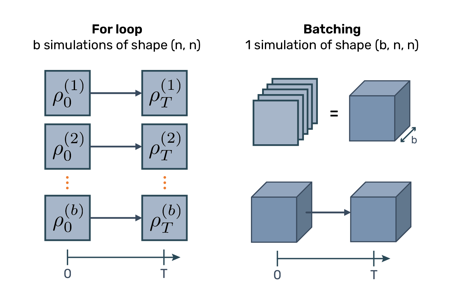Figure 1 / Schematic of batching. A number of simulations are ran as one in a higher-dimensional space instead of sequentially.

Benchmarking Dynamiqs

But just how much do GPUs and batching accelerate quantum simulations? In the table below, we show benchmarks of Dynamiqs against QuTiP over a set of 5 systems representative of typical problems in quantum optics and quantum information. These closed and open systems include a wide range of time-dependencies, Hilbert space sizes, number of modes, batching sizes, which are the main variables of performance. These benchmarks are run both on a standard cluster CPU and on an NVIDIA L40S GPU, dedicated to accelerated AI and high-performance computing. Comparison is made with QuTiP in its latest version, which is today the standard library for quantum simulations in Python, and on equal grounds by using the same tolerances and the default integration method of either library. Detailed benchmarks are open-source on the Dynamiqs GitHub, at this link.

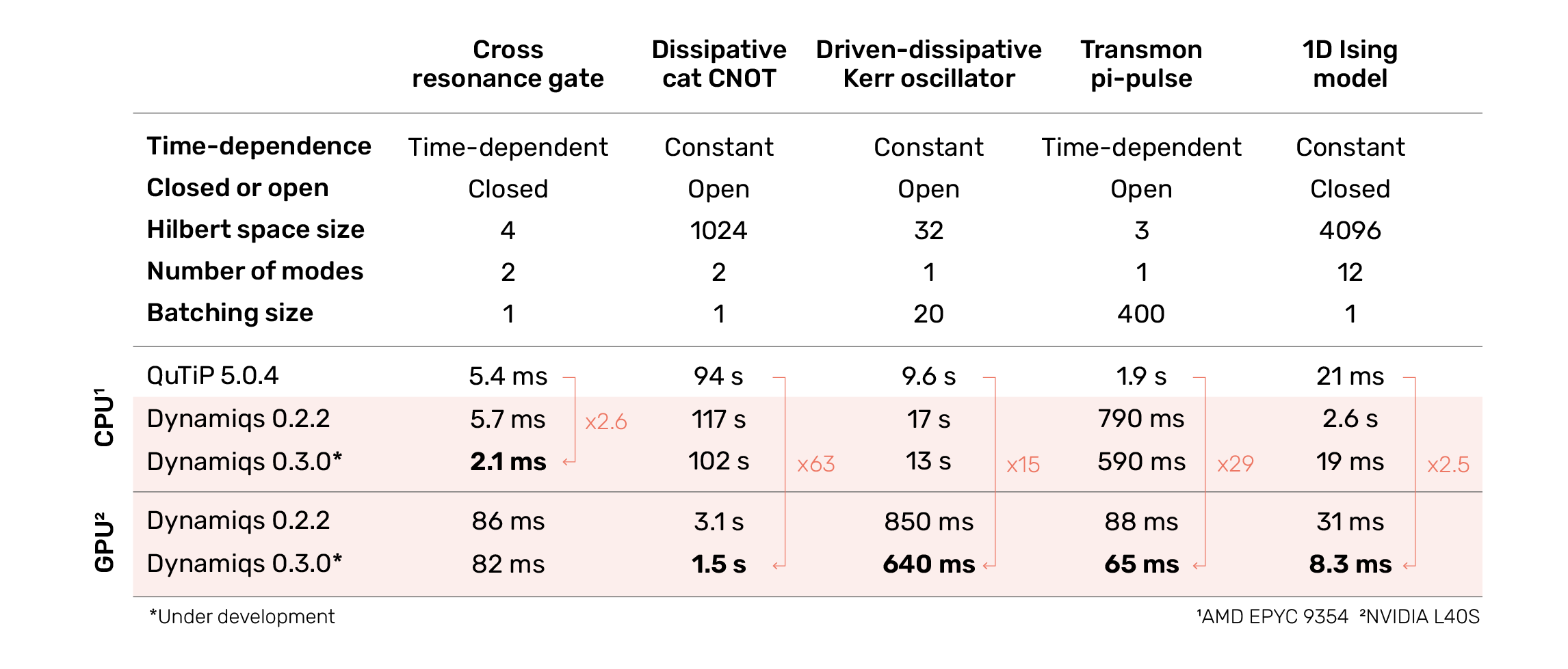Figure 2 / Benchmark table comparing Dynamiqs 0.2.2 (latest), Dynamiqs 0.3.0 (under development) and QuTiP 5.0.4 (latest) over a set of 5 representative simulations of quantum systems. GPU acceleration provides drastic speedups for large systems and for batching. On CPUs, Dynamiqs is on par with QuTiP, with speedup when benefiting from large batch sizes.

For all systems that we consider here, the latest release of Dynamiqs (v0.2.2) is at least on par with QuTiP and features up to a 30x speed increase on the dissipative cat CNOT benchmark by leveraging GPU acceleration. On Dynamiqs v0.3.0 (under development and planned for release before the end of 2024), the addition of the sparse representation of matrices provides a significant additional speedup, up to 60x on the same benchmark. In addition, the two benchmarks which benefit from batching show a 15x and 29x speedup respectively, while the benchmarks on small or closed systems show a more modest 2.5x speedup. Overall, such increases in performance are extremely beneficial in a day-to-day use and should open the door to a wide range of applications for researchers both in academia and industry.

Differentiability

Automatic differentiation has transformed the field of machine learning by enabling efficient explorations of massive parameter spaces in reasonable times. For quantum physics, we believe that it will be transformative. For instance, the ability to optimize the controls of quantum systems – known as quantum optimal control – can push the boundaries of fault-tolerant quantum computing by improving fidelities in the preparation, operation and readout of quantum devices. Quantum optimal control is often based on gradient descent which requires differentiable software such as Dynamiqs to compute gradients efficiently.

Another classic application of differentiability is parameter estimation. Here, the objective is to learn the model of a quantum physics experiment by fitting experimental observations with the simulation of this parametrized model. This is an essential application in the design and calibration of quantum devices, as a precise knowledge of the underlying hardware can drastically improve controlling a given system and designing its next generation.

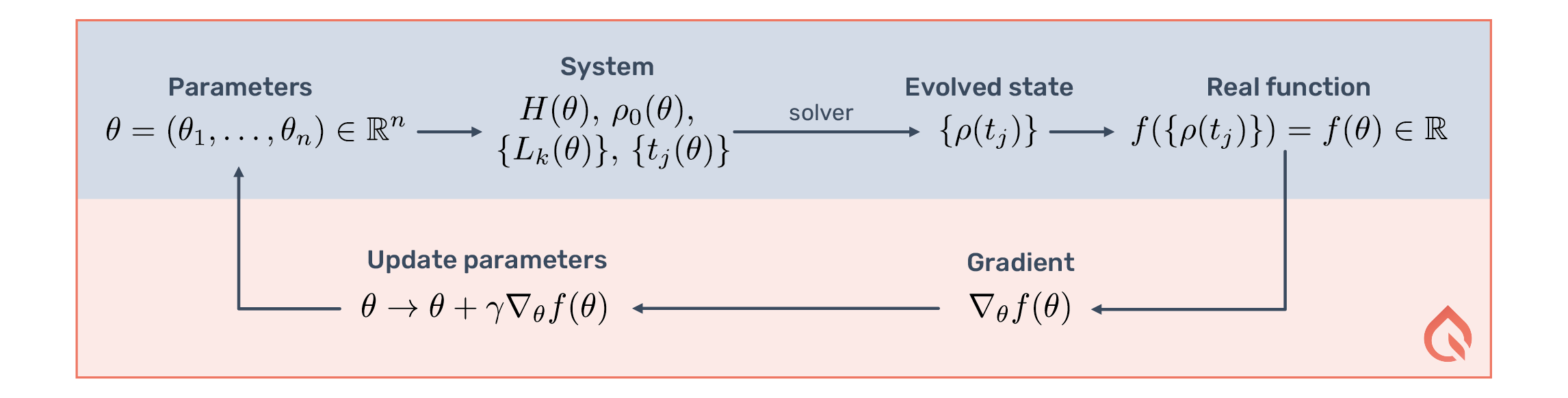Figure 3 / An optimization loop in Dynamiqs. Differentiability adds support for computing gradients in efficient time and memory, and thus closing the optimization loop.

In Dynamiqs, differentiability is again enabled by the underlying JAX codebase and by Diffrax, a state-of-the-art library for the integration of differential equations. Diffrax features memory-efficient automatic differentiation methods for large matrices, which is particularly relevant in the context of large open quantum systems or large batch sizes. To compute gradients against arbitrary parameters in Dynamiqs, the function to differentiate should be decorated with a @jax.grad. Subsequent calls to this decorated function will then proceed in two steps: a forward pass to evaluate the function, and a backward pass to evaluate its gradient against input parameters.

Importantly, the backward pass is equally time-consuming as the forward pass independently of the number of input parameters. This is a property of reverse-mode automatic differentiation for scalar-valued functions which makes gradient descents in large parameter spaces very effective. Once gradients are computed, performing the actual gradient descent can be achieved through libraries in the JAX ecosystem. For this task, the Optax library by Google DeepMind is a go-to.

Getting started

Dynamiqs makes it easy to dive into the world of GPU-accelerated and differentiable quantum simulations with just a few lines of code. Whether you’re new to quantum dynamics or a seasoned researcher, its simple API, close to that of QuTiP, and seamless compatibility with JAX allow you to focus on physics, not code. Here’s a basic example: simulating the preparation of a dissipative cat qubit.

Example: Preparing a Dissipative Cat Qubit

The following Python script demonstrates how to use Dynamiqs to simulate the time evolution of a quantum system. In this example, we prepare a dissipative cat qubit and visualize the evolution of its Wigner function.

import dynamiqs as dq
import jax.numpy as jnp

# simulation parameters
n = 24         # Hilbert space dimension
alpha = 2.0    # coherent state amplitude
kappa_2 = 1.0  # two-photon loss rate
tend = 2.0     # simulation end time
ntsave = 101   # number of time steps to save

# simulation inputs
a, adag = dq.destroy(n), dq.create(n)
H = 0.5j * alpha**2 * kappa_2 * (adag @ adag - a @ a)
jump_ops = [jnp.sqrt(kappa_2) * a @ a]
psi0 = dq.fock(n, 0)
tsave = jnp.linspace(0.0, tend, ntsave)

# run simulation
result = dq.mesolve(H, jump_ops, psi0, tsave)

# plot a GIF of the Wigner evolution
dq.plot.wigner_gif(result.states, ymax=2.5)

This code sets up a quantum system characterized by two-photon dissipation and simulates its evolution using the Lindblad master equation. Finally, it generates a GIF of the Wigner function over time, providing an intuitive visualization of the system’s state.

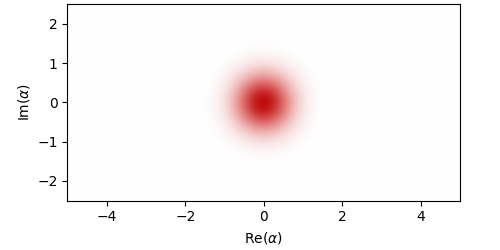
Figure 4 / Wigner of the preparation of a dissipative cat qubit, as generated by the code snippet above.

Run it Yourself!

• Install Dynamiqs via pip: pip install dynamiqs
• Make sure to configure your JAX environment to use GPUs if available. Switching to a GPU can be done with a simple call to dq.set_device.
• Check out more examples and the detailed documentation at dynamiqs.org or explore the source code on GitHub.

Conclusions

Dynamiqs is a powerful and accessible tool for GPU-accelerated and differentiable quantum simulations. By combining state-of-the-art performance with an accessible API, it addresses the growing demands of researchers. From simulating large systems to performing gradient-based optimizations, Dynamiqs is designed to simplify complex workflows while unlocking new possibilities in developing quantum technologies. It aims to be a fast and flexible building block for your quantum simulation projects.

Explore more at dynamiqs.org or dive into the source code on GitHub. Contributions are welcome, whether you’re adding features, reporting issues, or sharing your use cases. Together, let’s push the boundaries of quantum simulation!